Series: The Sequentia Lectures: Unlocking the Math of AI
Part 6: Advanced Architectures & Concepts
Lecture 56: Variational Autoencoders (VAEs): Learning the “Essence” of Data
Last time, we explored GANs, which learn to generate realistic data through a competitive “forger vs. detective” game. Today, we’ll look at another powerful generative model that takes a completely different, more introspective approach: the Variational Autoencoder (VAE).
Instead of a competition, a VAE works by learning to compress data down to its most essential features and then reconstruct it. In doing so, it learns the fundamental “recipe” or “essence” of the data it was trained on.
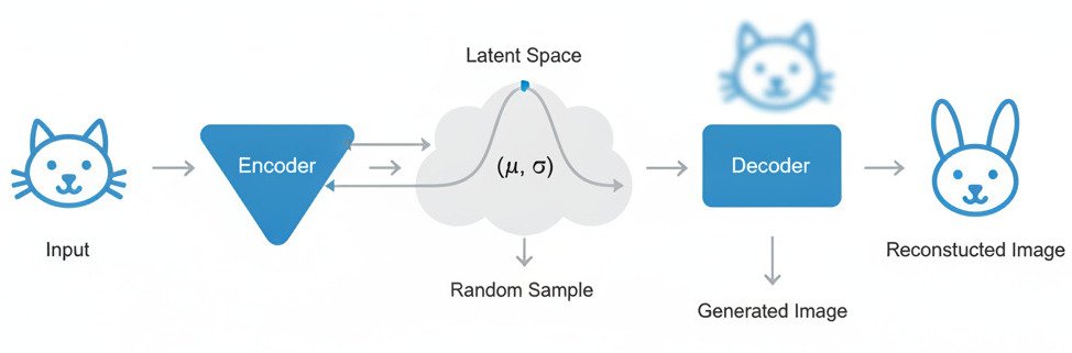
The Two-Part Architecture: Encoder and Decoder
A VAE, like a standard Autoencoder, is composed of two connected neural networks:
- The Encoder: This network’s job is to take a high-dimensional input, like an image, and compress it down into a much smaller, low-dimensional representation. It’s like reading a long, detailed book and summarizing it into a few key bullet points. This compressed representation is called the latent space.
- The Decoder: This network’s job is the reverse. It takes a point from the compressed latent space and attempts to reconstruct the original, high-dimensional input. It’s like taking the key bullet points and trying to write the entire book again from scratch.
The entire network is trained on a simple goal: the reconstructed output image should be as close as possible to the original input image.
The VAE’s Probabilistic Twist: The Latent Space
This is where a Variational Autoencoder differs from a standard one. A standard autoencoder might learn to map an input image to a single, precise point in the latent space. This is brittle; small changes in the input could lead to weird gaps or holes in the latent space.
A VAE is more sophisticated. It doesn’t just learn a single point; it learns a probability distribution for the latent space. Instead of saying, “This image of a cat maps to point X,” the encoder says, “This image of a cat maps to a small, fuzzy region centered around point X.”
Specifically, the encoder outputs two vectors for each input image: a mean vector (μ) and a standard deviation vector (σ). These two vectors define a simple Normal (Gaussian) distribution in the latent space. This is the “essence” of the input image, captured not as a single point, but as a region of possibilities.
From Learning to Generating
The training process forces the VAE to become an expert at compression and reconstruction.
- The Encoder must learn to capture only the most crucial, defining features of the input (e.g., “is it a cat?”, “what is its pose?”, “is it furry?”) and encode them into the parameters of the latent distribution.
- The Decoder must learn how to take these essential features and realistically flesh them out into a full image.
Once the VAE is trained, we can throw away the encoder and use the decoder as a generative model.
How? The latent space now represents a smooth, continuous map of all the “essences” of the data it has seen (e.g., all the possible “cat-nesses”). We can simply:
- Pick a random point from a standard Normal distribution in the latent space.
- Feed this random point into the Decoder.
- The Decoder, having learned how to turn these “essence” vectors into images, will generate a brand new, original image that looks like the data it was trained on!
Because the latent space is smooth and continuous, we can even perform “latent space arithmetic.” A point halfway between the latent representation of a “smiling man” and a “neutral-faced woman” might decode into an image of a “smiling woman.”
VAEs vs. GANs
VAEs and GANs are two different philosophies for generative modeling:
- GANs often produce sharper, more photorealistic images because the adversarial process forces the generator to perfect the fine details to fool the discriminator. However, they can be unstable and difficult to train.
- VAEs are much more stable to train and provide a well-structured, smooth latent space that is great for exploring variations in the data. The generated images can sometimes be slightly blurrier or more “dream-like” than GAN outputs.
The Variational Autoencoder is a beautiful and powerful idea. By forcing a model to learn the most compact and essential representation of data, it learns the very “essence” of that data, giving it the ability to dream up entirely new creations from that learned understanding.
