Series: The Sequentia Lectures: Unlocking the Math of AI
Part 6: Advanced Architectures & Concepts
Lecture 49: Recurrent Neural Networks (RNNs) 101: Giving AI a “Memory” for Sequences
So far, the networks we’ve discussed, including CNNs, have a limitation: they are feed-forward. Information flows in one direction, from input to output, and each decision is made independently. They have no memory of what came before. This is fine for classifying a static image, but what about data where order matters?
- How can a model understand a sentence if it forgets the beginning by the time it reaches the end?
- How can it predict the next value in a stock price series if it has no memory of the previous days’ prices?
To handle this sequential data, we need a new kind of architecture, one that has a form of memory. This is the Recurrent Neural Network (RNN).
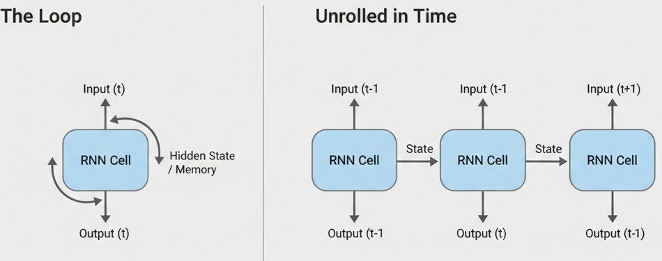
The Core Idea: The Loop of Memory
The ingenious innovation of the RNN is the loop.
In a standard feed-forward neuron, the output goes on to the next layer. In an RNN neuron (or “cell”), the output does two things:
- It goes on to the next layer to help make a prediction.
- It is fed back as an input to itself for the very next step in the sequence.
This loop allows the network to maintain a “memory” or a “state” that is passed along from one step to the next. The decision the network makes at Time Step T is influenced not just by the input at Time Step T, but also by a summary of all the information it has processed in the steps before.
Unrolling the Loop: An RNN in Action
To make this easier to visualize, we can “unroll” the loop through time. Imagine we have the sentence “The cat sat.” An RNN processes this word by word:
- Step 1 (Input: “The”):
- The network takes the vector for the word “The.”
- It processes this input and produces an output and a “hidden state” (its memory). Let’s call this State₁.
- Step 2 (Input: “cat”):
- The network now takes two inputs: the vector for the word “cat” AND the State₁ vector from the previous step.
- It combines these to produce a new output and a new hidden state, State₂, which now contains information from both “The” and “cat.”
- Step 3 (Input: “sat”):
- The network takes the vector for “sat” AND the State₂ vector.
- It processes these to produce the final output and State₃.
At each step, the hidden state acts as a running summary of the sequence so far. This “memory” allows the network to understand context. For example, when predicting the next word after “The cat sat on the…”, the hidden state’s memory of “cat” makes it much more likely to predict “mat” than “roof.”
The Power of Shared Weights (Again!)
Just like in CNNs, RNNs are incredibly efficient because they use shared weights. The same set of weights (the same “update rule” for the hidden state) is applied at every single time step.
The network doesn’t need to learn a separate set of rules for the first word, the second word, and the third word. It learns a single, recurrent rule for how to update its memory based on a new input. This allows it to process sequences of any length.
Applications of RNNs
This ability to process sequential information makes RNNs (and their more advanced successors like LSTMs and GRUs) the foundation for many powerful AI applications:
- Natural Language Processing (NLP): Machine translation, sentiment analysis, text generation, chatbots.
- Speech Recognition: Converting a sequence of audio signals into a sequence of words.
- Time Series Analysis: Stock price prediction, weather forecasting.
- Music Generation: Creating a new sequence of musical notes.
The Challenge: Vanishing Gradients (Again!)
While revolutionary, simple RNNs suffer from a major problem. When processing very long sequences, the error signal that is backpropagated “through time” can become very weak. This is the vanishing gradient problem, similar to the one we saw in deep feed-forward networks. It means the network struggles to learn long-range dependencies; it has a “short-term memory” and can forget the beginning of a long sentence.
This limitation led to the development of more sophisticated RNN architectures like LSTMs (Long Short-Term Memory) and GRUs (Gated Recurrent Units), which use special “gates” to more effectively control what information is kept in memory and what is forgotten. We’ll touch on these in a future lecture.
For now, the key takeaway is the power of the recurrent loop. It’s the simple yet brilliant mechanism that gives neural networks a memory, allowing them to move beyond static data and into the dynamic, ordered world of sequences.
