Lecture 47: The Math of a Convolution: A Sliding Window of Matrix Math

Series: The Sequentia Lectures: Unlocking the Math of AI
Part 6: Advanced Architectures & Concepts
Lecture 47: The Math of a Convolution: A Sliding Window of Matrix Math

In our last lecture, we introduced the core idea of a Convolutional Neural Network (CNN): small “filters” that slide across an image to detect features. Today, we’re going to zoom in and look at the precise mathematical operation that makes this happen. This operation is called a convolution.

While the term might sound complex, the underlying math is a beautiful and efficient application of the linear algebra we’ve already learned. It’s essentially a series of dot products performed in a sliding window.

Setting the Scene: The Image and the Filter

Let’s imagine our data in its numerical form:

• The Input Image: A large matrix (a 2D grid) of pixel values. For a grayscale image, a pixel value of 0 might be black and 255 might be white.
• The Filter (or Kernel): A small matrix of weights, typically 3×3. These weights are the parameters that the network learns.

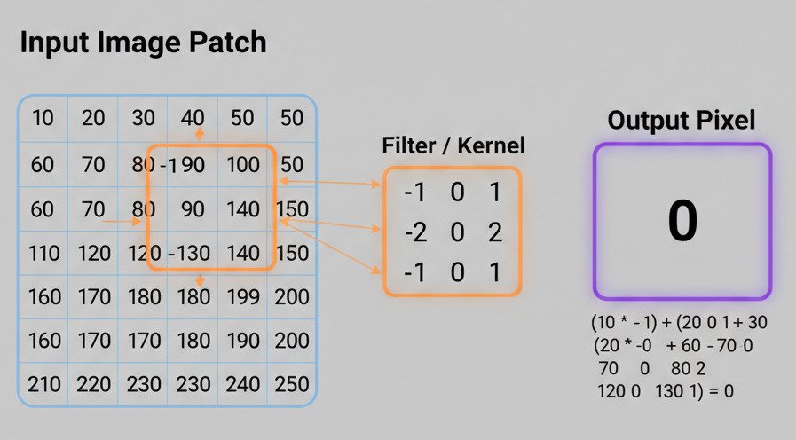
Let’s use a simple example. Here is a small 5×5 patch of an image and a 3×3 filter designed to detect a simple diagonal line from top-left to bottom-right.

Input Image Patch (5×5):

10  10  10  80  80
10  10  80  80  80
10  80  80  80  10
80  80  80  10  10
80  80  10  10  10

Filter / Kernel (3×3):

10   0   0
 0  10   0
 0   0  10

This filter has large weights along its main diagonal, so it will “light up” when it encounters a similar diagonal pattern in the image.

The Convolution Operation: A Step-by-Step Dot Product

The convolution operation is a “sliding window” process. Here’s what happens:

1. Placement: The 3×3 filter is placed over the top-left 3×3 corner of the image.
2. Element-wise Multiplication: Each number in the filter is multiplied by the number in the image pixel directly underneath it.
3. Summation (The Dot Product!): All nine of the resulting products are summed up to produce a single number. This is effectively the dot product of the flattened filter vector and the flattened image patch vector.
4. Output: This single number becomes the top-left pixel in our new Feature Map.
5. Slide: The filter then slides one position to the right (this is called a “stride” of 1), and the entire process repeats to calculate the next pixel in the feature map.
6. Repeat: The filter continues to slide across the entire image, row by row, filling in the feature map pixel by pixel.

Let’s calculate the first value for our example:

• Top-Left Image Patch: [10, 10, 10], [10, 10, 80], [10, 80, 80]
• Filter: [10, 0, 0], [0, 10, 0], [0, 0, 10]
• Calculation:
  (10*10) + (10*0) + (10*0) +
  (10*0) + (10*10) + (80*0) +
  (10*0) + (80*0) + (80*10) = 100 + 0 + 0 + 0 + 100 + 0 + 0 + 0 + 800 = **1000**
• The top-left pixel of our feature map has a high value (1000), indicating a strong match for the diagonal pattern in that spot.

If the filter were placed over a patch with no diagonal pattern, the resulting dot product would be a very small number, indicating a low activation.

The Power of Translation Invariance

Why is this sliding dot product so powerful? Because it achieves translation invariance.

The weights in our filter ([10, 0, 0], [0, 10, 0], …) are the same regardless of where the filter is on the image. This means the filter is equally capable of detecting a diagonal line in the top-left corner, the center, or the bottom-right corner. It learns to recognize a feature, and then the convolution operation allows it to find that feature anywhere.

This is a massive advantage over the fully connected networks we discussed earlier, which would have to learn separate weights for detecting a diagonal line in every single possible position on the image. The convolution shares these learned weights across the entire image, making the process incredibly efficient and robust to the position of objects.

The convolution, therefore, is not just a mathematical curiosity. It is the elegant, efficient, and powerful operation that gives CNNs their ability to “see” patterns in a way that mimics our own visual system—by applying a consistent set of feature detectors across our entire field of view.