Series: The Sequentia Lectures: Unlocking the Math of AI
Part 5: Core Machine Learning in Action
Lecture 37: Logistic Regression: Predicting “Yes” or “No” with a Squiggly Line (Sigmoid)
In our last lecture, we successfully built our first machine learning model, Linear Regression. It’s a fantastic tool for predicting continuous values, like the price of a house or a student’s test score.
But many of the most interesting questions in the world aren’t about “how much?”; they’re about “which one?”.
- Is this email Spam or Not Spam?
- Will this customer Buy or Not Buy?
- Is this tumor Malignant or Benign?
These are classification problems, where we need to predict a category, often a binary (Yes/No) outcome. A straight line from linear regression isn’t the right tool for this. Why? Because a line can output any value from negative infinity to positive infinity. How do we interpret a prediction of “-50” or “120” when we just want a “Yes” or “No”?
We need a new kind of model. We need Logistic Regression.
The Core Idea: From a Line to a Probability
Logistic Regression is a clever and elegant adaptation of Linear Regression. It starts in the exact same way: by calculating a score using a linear equation, just like y = mx + b (or for multiple features, a weighted sum/dot product).
Score = w₁x₁ + w₂x₂ + … + b
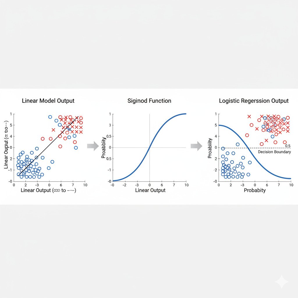
This score can still be any number. But here’s the magic trick: Logistic Regression takes this raw score and passes it through a special “squashing” function called the Sigmoid Function (or Logistic Function).
The Sigmoid Function: The “S”-Curve of Probability
The Sigmoid function is a beautiful S-shaped curve. Its special property is that it can take any real number as input and “squash” its output to be a value strictly between 0 and 1.
- Very large positive inputs get squashed to be very close to 1.
- Very large negative inputs get squashed to be very close to 0.
- An input of 0 gets mapped to exactly 0.5.
By passing our linear score through the sigmoid function, we are no longer predicting a raw number; we are predicting a probability.
Probability = Sigmoid(Score)
This probability is our model’s confidence that the outcome is “Yes” (or the “1” class).
- If the sigmoid output is 0.9, our model is 90% confident the answer is “Yes.”
- If the sigmoid output is 0.1, our model is 10% confident the answer is “Yes” (or, equivalently, 90% confident the answer is “No”).
Making the Final Decision: The Threshold
To get our final “Yes” or “No” classification, we simply apply a decision threshold to this probability, which is usually set at 0.5.
- If Probability >= 0.5, we predict “Yes” (Class 1).
- If Probability < 0.5, we predict “No” (Class 0).
So, the entire process is:
- Calculate a linear score from the inputs and weights.
- Pass this score through the Sigmoid function to get a probability between 0 and 1.
- Apply a 0.5 threshold to this probability to make the final binary classification.
How Does It Learn? Minimizing “Surprise”
We can’t use Mean Squared Error (MSE) as our cost function anymore, because our predictions are now probabilities. Instead, for classification problems, we use a cost function rooted in information theory, like the Cross-Entropy Loss we discussed in Lecture 33.
The intuition is the same: the cost function measures how “surprised” our model is by the true answer. If the true answer is “Yes” (1) and our model confidently predicted a probability of 0.9, the surprise (cost) is low. If it predicted 0.1, the surprise (cost) is very high.
We then use Gradient Descent, just as before, to find the weights (w) and bias (b) that minimize this cross-entropy cost across our entire dataset. The model learns to adjust its internal linear equation so that when fed through the sigmoid, the resulting probabilities are as close as possible to the true outcomes.
Logistic Regression is the foundational algorithm for classification. It beautifully combines the linear model we already know with a clever non-linear “squashing” function to turn a simple score into a meaningful probability, forming the basis for many more complex classification models in AI.
