Lecture 36: Linear Regression: Drawing the “Best” Line Through Data

Series: The Sequentia Lectures: Unlocking the Math of AI
Part 5: Core Machine Learning in Action
Lecture 36: Linear Regression: Drawing the “Best” Line Through Data

Welcome to Part 5 of the Sequentia Lectures! We’ve spent weeks assembling our mathematical toolkits: Linear Algebra to structure our data, Calculus to measure change, and Statistics to reason under uncertainty. Now, it’s time to put it all together and build our very first, and arguably most fundamental, machine learning model: Linear Regression.

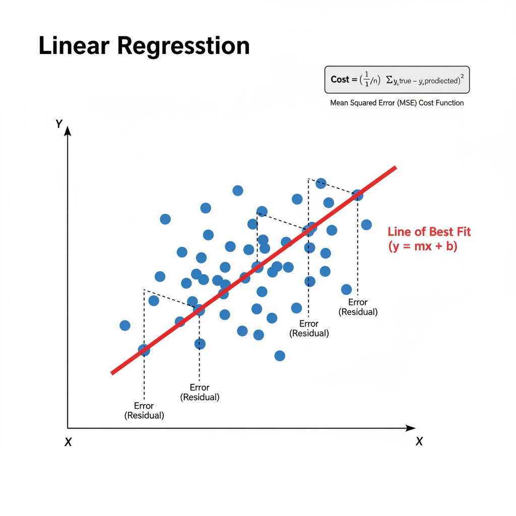
The goal of linear regression is simple and intuitive: given a scatter plot of data points, how do we find the single straight line that best “fits” or summarizes the underlying trend in that data?

The Puzzle: Predicting a Value

Imagine we have a simple dataset that tracks two variables: the number of hours a student studies, and the score they get on a test.

• Student 1: Studies 2 hours, scores 65.
• Student 2: Studies 4 hours, scores 75.
• Student 3: Studies 5 hours, scores 85.

We can plot this on a 2D graph. Our task is to draw a line that we can use to predict the test score for a student who studies for, say, 3 hours.

Step 1: Representing the Problem with Linear Algebra

First, we need to define our model. A straight line is defined by the simple equation:

y = mx + b

Where:

• y is the output we want to predict (the test score).
• x is our single input feature (hours studied).
• m is the slope of the line (how much the score increases for each extra hour of study).
• b is the y-intercept (the score a student would get for studying 0 hours).

Our model’s “parameters”—the knobs we can turn to change the model—are m and b. The entire goal of training is to find the best possible values for m and b. We can represent these parameters in a vector, and our data in matrices, exactly as we learned in Part 2.

Step 2: Defining “Best” with a Cost Function (Calculus & Statistics)

How do we know if one line is “better” than another? We need to measure the error. As we discussed in Lecture 20, a great way to do this for regression problems is the Mean Squared Error (MSE) cost function.

For each data point, we:

1. Use our current line (y = mx + b) to make a prediction for a given x.
2. Measure the vertical distance between our predicted y and the actual y. This is the error.
3. Square this error.
4. The MSE is the average of these squared errors across all our data points.

Our cost function, J(m, b), takes our parameters m and b as input and gives us a single number representing the total error of our line. Our goal is to find the m and b that make J(m, b) as small as possible.

Step 3: Finding the Best Line with Gradient Descent (Optimization)

We now have our “error landscape,” where the “location” is defined by the values of m and b, and the “elevation” is the MSE cost. To find the bottom of this valley, we use Gradient Descent.

1. Initialize: Start with random guesses for m and b. This gives us a starting line, which is probably a terrible fit.
2. Calculate the Gradient: We compute the partial derivatives of our cost function J(m, b) with respect to both m and b.
   • The partial derivative with respect to m (∂J/∂m) tells us how the error changes if we slightly change the slope.
   • The partial derivative with respect to b (∂J/∂b) tells us how the error changes if we slightly change the intercept.
   • These two values form our gradient vector: ∇J = [ ∂J/∂m, ∂J/∂b ].
3. Update the Parameters: We take a small step in the direction opposite to the gradient to update our m and b:
   • m_new = m_old – (learning_rate * ∂J/∂m)
   • b_new = b_old – (learning_rate * ∂J/∂b)
4. Repeat: We go back to Step 2 and repeat this process. With each iteration, our line y = mx + b will shift and tilt, getting progressively closer to the data points, minimizing the error.

After many iterations, the algorithm will converge on the optimal values for m and b, giving us the single “line of best fit” that minimizes the Mean Squared Error. We have officially “trained” our first machine learning model!

Putting It All Together

Linear Regression is the perfect culmination of our journey so far:

• We framed the problem using the Linear Algebra of lines, vectors ([m, b]), and data points.
• We chose a Cost Function (MSE), a concept rooted in statistics, to quantify our model’s error.
• We used the tools of Calculus (derivatives) to find the gradient of our cost function.
• We used an Optimization algorithm (Gradient Descent) to iteratively follow that gradient and find the best possible parameters.

It’s a beautiful symphony of all three mathematical fields working together to solve a single, tangible problem. In our next lecture, we’ll extend this idea to handle more than just one input feature, moving into the world of Multiple Linear Regression.