Series: The Sequentia Lectures: Unlocking the Math of AI
Part 4: The AI Toolkit: Probability & Statistics
Lecture 34: KL Divergence: Measuring the “Distance” Between Two Beliefs
In our last lecture, we learned about Entropy, a way to measure the uncertainty or “surprise” within a single probability distribution. We also touched upon Cross-Entropy, which measures the “surprise” our model feels when it sees the true data.
Now, let’s ask a related but different question: how can we directly compare two different probability distributions and measure exactly how different they are? For instance, how can we quantify the “distance” between our model’s set of beliefs (its predicted distribution) and the actual, true distribution of the data?
The tool for this is a fundamental concept from information theory called Kullback-Leibler Divergence, or simply KL Divergence.
What is KL Divergence?
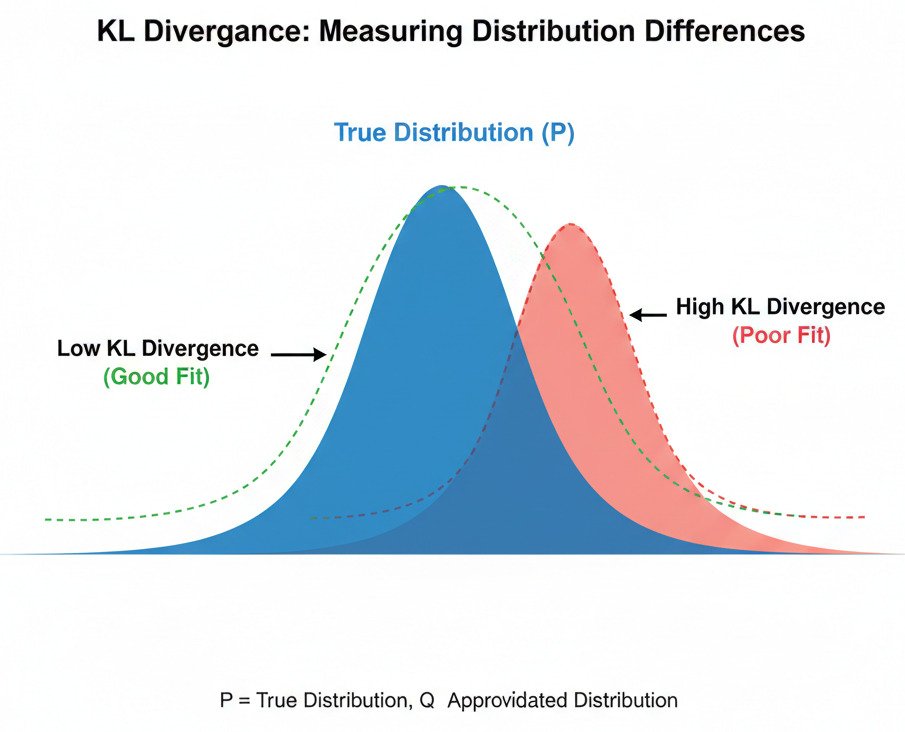
KL Divergence measures the “information lost” or “extra surprise” we encounter when we use an approximated probability distribution (Q) to represent a true probability distribution (P).
Imagine you are an expert on animal populations in a specific forest (this is the “true” distribution, P). You know that the animals are 60% squirrels, 30% rabbits, and 10% deer.
- P = { Squirrel: 0.6, Rabbit: 0.3, Deer: 0.1 }
Now, an AI model is trying to learn this distribution. Its current, imperfect belief is represented by distribution Q.
- Q = { Squirrel: 0.5, Rabbit: 0.4, Deer: 0.1 }
KL Divergence gives us a single number that tells us how “bad” Q is as an approximation of P.
The Intuition: A Measure of Inefficiency
Think of KL Divergence as a measure of inefficiency in communication. If you were to design an optimal code (like Morse code) based on the true frequencies of animals (P), you would use very short codes for squirrels and longer codes for deer.
If you then used this optimal code but the animals actually appeared with the frequencies of Q, your communication would be slightly less efficient. KL Divergence quantifies the average number of extra bits of information you would need to transmit messages because of this mismatch.
- If Q is identical to P, the KL Divergence is 0. There is no information lost, no extra surprise. Your approximation is perfect.
- If Q is very different from P, the KL Divergence is a large positive number. A lot of information is lost; your approximation is poor, and you’ll be constantly surprised.
An Important Quirk: It’s Not a True “Distance”
One crucial property of KL Divergence is that it is asymmetric.
KL(P || Q) ≠ KL(Q || P)
The “distance” from P to Q is not the same as the “distance” from Q to P. This is why we often refer to it as a “divergence” rather than a “distance.” It measures the information lost when approximating P with Q, which is a one-way street.
KL Divergence in AI: Training Generative Models
While KL Divergence is mathematically related to Cross-Entropy (in fact, Cross-Entropy is just Entropy + KL Divergence), it has a particularly important role in a class of AI models called Generative Models.
These models (like Variational Autoencoders or VAEs) aim to learn the entire, complex probability distribution of the training data. For example, a model trained on thousands of faces learns the “distribution of what a face looks like.” It can then be used to generate new, realistic-looking faces by sampling from this learned distribution.
During training, the goal is often to minimize the KL Divergence between the model’s internal, simplified distribution and the true (but unknown) distribution of the real data. By pushing the KL Divergence towards zero, we are forcing our model’s “beliefs” about the world to become as close as possible to the actual “reality” of the data. The model learns to generate data that is “less surprising” and more faithful to the original source.
In essence, KL Divergence provides a powerful cost function for any AI task where the goal isn’t just to predict a single label, but to learn and replicate a complete, complex data distribution. It’s the mathematical tool that allows us to measure how well our AI’s “worldview” matches the real world.
