Series: The Sequentia Lectures: Unlocking the Math of AI
Part 4: The AI Toolkit: Probability & Statistics
Lecture 30: Mean, Variance, & Standard Deviation: The Core Stats of Your Data
Imagine you’re handed a giant spreadsheet with thousands of numbers—perhaps the test scores of every student in a district, or the daily temperatures for a city over the last decade. Staring at the raw data is overwhelming. How can we begin to make sense of it all?
Before we can build complex AI models, we must first learn to describe our data. We need a simple, concise summary that captures its essential characteristics. This is the job of descriptive statistics, and the three most fundamental measures are the Mean, Variance, and Standard Deviation.
The Mean: Finding the “Center of Gravity”
The mean, or average, is the most common measure of the “central tendency” of a dataset. It tells us where the “center of gravity” of our data lies.
The calculation is simple and familiar: you sum up all the values in your dataset and then divide by the number of values.
Mean (μ) = (Sum of all values) / (Number of values)
If we have the test scores [85, 90, 75, 95, 80], the mean is:
(85 + 90 + 75 + 95 + 80) / 5 = 425 / 5 = 85
The mean gives us a single number that represents the “typical” value in our dataset. In our lectures on probability distributions, the mean is what determines the center of the bell curve. It’s our first and most important piece of information about a dataset’s location on the number line.
Variance & Standard Deviation: Measuring the “Spread”
Knowing the center is great, but it doesn’t tell the whole story. Consider two different classes that both have an average test score (mean) of 85.
- Class A Scores: [84, 85, 85, 86, 85]
- Class B Scores: [60, 100, 90, 70, 105]
While their average is the same, the nature of these datasets is completely different! Class A is very consistent, with all scores clustered tightly around the mean. Class B is wildly spread out. We need a way to quantify this “spread,” and that’s where variance and standard deviation come in.
Variance (σ²): The Average Squared Difference
Variance measures, on average, how far each data point is from the mean. The calculation is a bit more involved:
- Calculate the mean of the data.
- For each data point, subtract the mean and then square the result. (This squaring step ensures all differences are positive and penalizes points that are far from the mean).
- Calculate the average of all these squared differences.
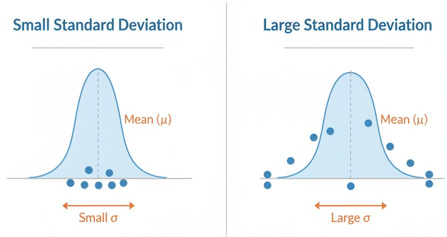
A small variance means the data points are tightly clustered. A large variance means they are widely spread out.
Standard Deviation (σ): The Intuitive Spread
The variance gives us a great measure of spread, but its units are squared (e.g., “dollars squared”), which can be hard to interpret. To fix this, we simply take the square root of the variance. This gives us the standard deviation.
The standard deviation is a number that represents a “typical” or “standard” amount of deviation from the average. It’s measured in the same units as the original data, making it much more intuitive.
- If the mean house price is $500k and the standard deviation is $50k, it gives us a good sense of the typical price range.
- In our class example, Class A would have a very small standard deviation, while Class B’s would be very large.
In a Normal (bell curve) distribution, roughly 68% of all data points will lie within one standard deviation of the mean, and about 95% will lie within two standard deviations.
Why This Matters for AI
These simple descriptive stats are the first things a data scientist calculates when they receive a new dataset.
- Understanding Data: They provide a quick, high-level summary of each feature. Is the data centered around zero? Is it widely spread out or tightly clustered?
- Data Preprocessing (Standardization): Many AI algorithms work best when the input features have a mean of 0 and a standard deviation of 1. A process called “standardization” uses the mean and standard deviation to rescale the data, which can significantly improve model training.
- Detecting Anomalies: If a new data point is many standard deviations away from the mean, it’s likely an outlier or an anomaly that might require special attention.
The mean, variance, and standard deviation are our fundamental tools for taking a chaotic cloud of raw data and distilling it down to its most essential properties: its center and its spread. They are the first step in turning data into information.
