Series: The Sequentia Lectures: Unlocking the Math of AI
Part 6: Advanced Architectures & Concepts
Lecture 58: The Math of Q-Learning: A Simple Way to Learn the “Value” of Actions
In our last lecture, we introduced Reinforcement Learning (RL) as a process of an agent learning through trial, error, and rewards. The agent’s goal is to learn a “policy”—a strategy that tells it which action to take in any given state to maximize its total future reward.
But how does it actually learn this policy? How does it decide if an action is “good” or “bad”? One of the earliest and most foundational algorithms for this is Q-Learning. The “Q” stands for “Quality,” and the algorithm is all about learning the quality, or value, of taking a specific action in a specific state.
Introducing the Q-Table: A Cheat Sheet for Our Agent
At the heart of simple Q-learning is a table, often called a Q-table. This table is the agent’s “brain” or “cheat sheet.”
- The rows of the table represent all the possible states the agent can be in.
- The columns represent all the possible actions the agent can take.
- Each cell in the table, Q(state, action), will eventually hold a number: the Q-value.
The Q-value, Q(s, a), represents the total future reward the agent can expect to get if it starts in state s, takes action a, and then continues to act optimally from that point onwards. It’s not just the immediate reward; it’s a prediction of the entire long-term, cumulative reward.
Initially, this Q-table is filled with zeros. The agent knows nothing. The “learning” process is all about exploring the environment and gradually filling in this table with better and better estimates of the true Q-values.
The Q-Learning Algorithm: Exploring and Updating
The Q-learning agent learns by moving through the environment and updating its Q-table using a special update rule. Here’s the loop:
- Observe: The agent is in a certain state (s).
- Choose an Action (a): The agent decides which action to take. At the beginning, it might choose randomly to explore. As it learns, it will more often choose the action with the highest Q-value for its current state (exploiting what it already knows). This is the exploration vs. exploitation trade-off.
- Perform Action & Observe: The agent performs the action and the environment gives back two things:
- The immediate reward (r).
- The new_state (s’).
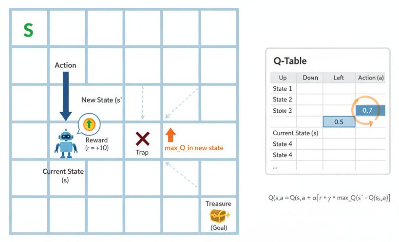
- Update the Q-Table: This is the core of the algorithm. The agent updates the Q-value for the state-action pair it just experienced (Q(s, a)) using the Bellman equation, a cornerstone of reinforcement learning. The simplified update rule looks like this:
New Q(s, a) = Old Q(s, a) + learning_rate * [ (reward + discount_factor * max_Q_in_new_state) – Old Q(s, a) ]
Let’s break that down:
- Old Q(s, a): What we used to think the value was.
- learning_rate: How much we want to update our old value based on new information (just like in Gradient Descent!).
- reward: The immediate treat we just got.
- discount_factor (gamma, γ): A number between 0 and 1 that represents how much we value future rewards compared to immediate ones. A low gamma makes the agent “short-sighted,” while a high gamma makes it prioritize long-term gains.
- max_Q_in_new_state: The agent looks at the new_state (s’) it just landed in and finds the best possible Q-value it could get by taking the best action from that new state. This is its “estimate of future reward.”
- The term in the [ … ] brackets represents the “learning error”—the difference between our new, updated estimate of the value and our old one.
The agent is essentially updating its old belief (Old Q(s, a)) by nudging it a little bit in the direction of a new, more informed belief based on the real reward it just received plus its best guess of what the future looks like from its new position.
Learning the Optimal Policy
The agent repeats this loop thousands or millions of times, exploring every corner of its environment. With each step, the Q-values in the table get more and more accurate. The values “propagate” backward from high-reward states. An agent might stumble upon a treasure (high reward) at the end of a maze. The Q-value for the state-action pair that led to the treasure gets updated. On the next run, the state before that will see that its “estimate of future reward” is now higher, so its Q-value gets updated, and so on.
Once the Q-table is well-trained, the agent’s “policy” is simple: in any given state, just choose the action that has the highest Q-value. This table has become a complete guide to navigating the environment for maximum reward.
While this simple table-based Q-learning only works for environments with a finite (and small) number of states and actions, it provides the fundamental concept for more advanced methods like Deep Q-Networks (DQN), where a neural network is used to predict the Q-values instead of storing them in a table, allowing agents to learn in incredibly complex environments like video games.
