Series: The Sequentia Lectures: Unlocking the Math of AI
Part 6: Advanced Architectures & Concepts
Lecture 50: The Vanishing & Exploding Gradient Problem: Why Simple RNNs Fail
In our last lecture, we celebrated the ingenious loop of the Recurrent Neural Network (RNN), which gives it a form of “memory” to process sequential data. It seems like a perfect solution. However, in practice, the simple RNN architecture suffers from a critical, often fatal, flaw that makes it struggle with long-term memory.
This flaw is known as the Vanishing and Exploding Gradient Problem. To understand it, we need to revisit our old friend from calculus: the Chain Rule.
Backpropagation Through Time
When an RNN learns, it uses a version of backpropagation called Backpropagation Through Time (BPTT). After processing a sequence and calculating the final error, the error signal needs to be passed backwards, not just through layers, but backwards through the time steps of the “unrolled” network.
Imagine our unrolled network from the last lecture:
… -> Cell (t-1) -> Cell (t) -> Cell (t+1) -> … -> Final Error
To update the weights, we need to know how a change at Time Step (t-1) affects the final error, which might occur many steps later. According to the Chain Rule, we do this by multiplying the derivatives at each successive step.
The derivative of the error with respect to the state at Time Step (t-1) is roughly:
(Derivative at t+1) * (Derivative at t) * (Derivative at t-1)
And what is this “derivative at each step”? It’s largely determined by the recurrent weight matrix—the shared set of weights that is applied over and over again in the loop.
The Problem: Repeated Multiplication
Herein lies the problem. We are multiplying the same matrix (or its derivatives) by itself, over and over again, for as many time steps as we need to go back. What happens when you repeatedly multiply a number by another number?
- If the number is less than 1 (e.g., 0.8): The result shrinks towards zero very quickly.
0.8 * 0.8 = 0.64
0.8 * 0.8 * 0.8 = 0.512
0.8¹⁰ ≈ 0.1 - If the number is greater than 1 (e.g., 1.2): The result grows uncontrollably.
1.2 * 1.2 = 1.44
1.2 * 1.2 * 1.2 ≈ 1.728
1.2¹⁰ ≈ 6.2
The same principle applies to the gradients being passed back through the RNN.
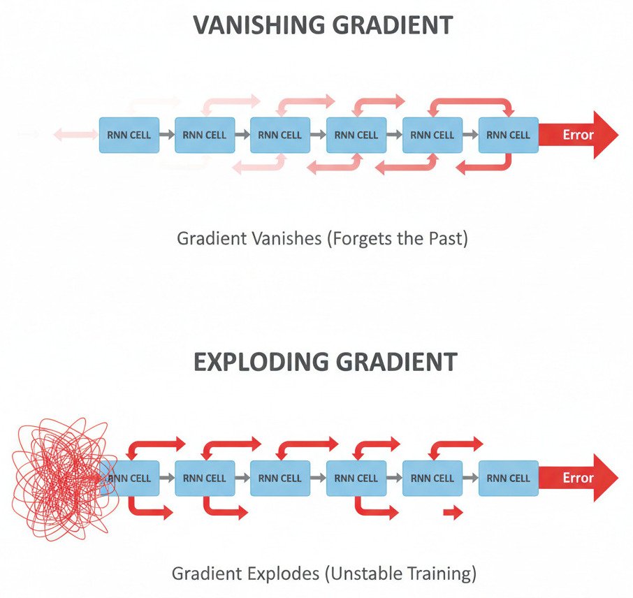
1. The Vanishing Gradient
If the weights in our recurrent matrix are small (and the derivatives of our activation function are less than 1), then as we backpropagate the error signal through many time steps, it gets multiplied by a number less than 1 over and over again. The gradient signal shrinks exponentially, quickly vanishing to near zero.
- The Consequence: By the time the error signal reaches the early time steps, it’s so minuscule that it provides no useful information. The network is unable to learn the connection between events that are far apart in the sequence.
- The Effect: The RNN effectively has a “short-term memory.” It can learn that in the phrase “New York,” the word “York” often follows “New.” But it will fail to learn the grammatical dependency in a long sentence like, “The cats, which I saw playing in the yard all morning, are now sleeping.” The network forgets that the subject was plural (“cats”) by the time it needs to choose the verb (“are” vs. “is”).
2. The Exploding Gradient
Conversely, if the weights in our recurrent matrix are large, the gradient signal gets multiplied by a number greater than 1 over and over again. The signal grows exponentially until it becomes astronomically large, or explodes.
- The Consequence: These enormous gradients cause the weight updates to be huge and erratic. It’s like taking a giant, reckless leap in Gradient Descent.
- The Effect: The training process becomes unstable, and the model fails to learn anything meaningful. The cost function might fluctuate wildly or return NaN (Not a Number). (While easier to detect than vanishing gradients, it’s still a critical failure).
The Need for a Smarter Memory
The vanishing gradient problem, in particular, was a major obstacle that prevented simple RNNs from being effective on tasks requiring long-term memory. The architecture itself was fighting against the learning algorithm.
This fundamental limitation directly led to the development of more sophisticated recurrent architectures designed to combat this problem. These models, most notably Long Short-Term Memory (LSTM) and Gated Recurrent Units (GRU), don’t just pass the entire hidden state through a simple transformation. They use a system of “gates”—internal mechanisms that learn to selectively add new information, forget old, irrelevant information, and pass through important long-term memories.
These gated architectures are the topic of our next lecture, and they are the innovation that truly unlocked the power of recurrent networks for complex sequential tasks.
