Series: The Sequentia Lectures: Unlocking the Math of AI
Part 6: Advanced Architectures & Concepts
Lecture 46: Convolutional Neural Networks (CNNs) 101: How AI “Sees” with Filters
In our previous lectures, we built a standard “Multi-Layer Perceptron” where every neuron in one layer is connected to every neuron in the next. While powerful, this approach struggles with images. If you have a high-definition photo, connecting every pixel to every neuron in a hidden layer would result in billions of weights, making the model slow, memory-hungry, and prone to overfitting.
To solve this, AI researchers looked to nature. Specifically, they looked at the human visual cortex. They discovered that our brains don’t look at every pixel of a scene at once. Instead, specialized groups of neurons focus on small, local patches, looking for specific patterns like edges or curves.
This insight led to the creation of the Convolutional Neural Network (CNN).
The Magic of the Filter (Kernel)
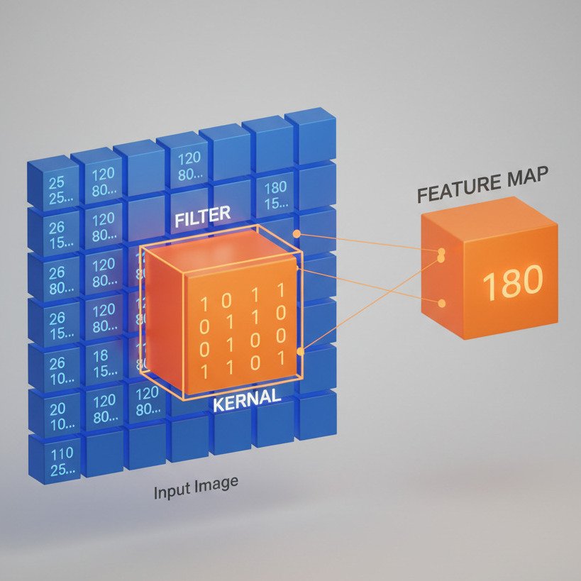
The core building block of a CNN is the Filter (also called a Kernel). Instead of a massive matrix that looks at the whole image, a filter is a tiny matrix—often just 3×3 or 5×5 pixels in size.
Imagine holding a small magnifying glass over a large photograph. You slide that glass across the image, row by row, looking for one specific thing—for example, a vertical edge.
The Math of Convolution
As the filter “slides” across the image, it performs a simple mathematical operation at every stop: the dot product.
- The filter is placed over a 3×3 patch of pixels.
- Each pixel value in that patch is multiplied by the corresponding value in the filter.
- All 9 results are summed up into a single number.
This single number represents how strongly that specific feature (like a vertical edge) exists in that specific patch of the image. After the filter has slid across the entire image, it produces a new grid of numbers called a Feature Map.
Specialized Detectors
A CNN doesn’t just use one filter. It uses dozens or hundreds in every layer!
- Filter 1 might be a vertical edge detector.
- Filter 2 might be a horizontal edge detector.
- Filter 3 might look for a specific color gradient.
- Filter 4 might look for a sharp corner.
Each filter creates its own “Feature Map,” highlighting where its specific pattern appears in the original image.
Efficiency Through “Shared Weights”
Here is the genius of the CNN: because we use the same 3×3 filter to scan the entire image, the number of parameters is incredibly small. A 3×3 filter only has 9 weights, regardless of how big the image is!
This concept is called Shared Weights. It assumes that if a feature (like an edge) is important to find in the top-left corner, it’s just as important to find in the bottom-right. This makes CNNs incredibly efficient and allows them to recognize objects regardless of where they appear in the frame (a property called “translation invariance”).
The Hierarchy of Vision
Just like the multi-layer networks we discussed in Lecture 40, CNNs work in a hierarchy:
- Early Layers: Use simple filters to find basic edges and textures.
- Middle Layers: Take those edge-maps as inputs and use new filters to find more complex shapes like circles, eyes, or ears.
- Deep Layers: Combine those shapes to identify complex objects like “Face,” “Car,” or “Dog.”
By replacing massive, “fully connected” layers with these small, sliding filters, CNNs allow AI to process visual information with incredible speed and accuracy. They don’t just “see” numbers; they “see” features, building up an understanding of the world one edge and corner at a time.
In our next lecture, we’ll look at the “cleanup crew” of the CNN: the Pooling layer.
