Lecture 40: Building a Simple Neural Network: Stacking Neurons into Layers

Series: The Sequentia Lectures: Unlocking the Math of AI
Part 5: Core Machine Learning in Action
Lecture 40: Building a Simple Neural Network: Stacking Neurons into Layers

We’ve arrived at a major milestone. We’ve studied the individual components: the single neuron (the Perceptron), the matrix of weights that connects them, and the non-linear Activation Function (like ReLU) that gives them their power.

Now, it’s time to assemble them. How do we go from a single neuron to a Neural Network? We do it by stacking these simple computational units into layers.

The Anatomy of a Multi-Layer Perceptron (MLP)

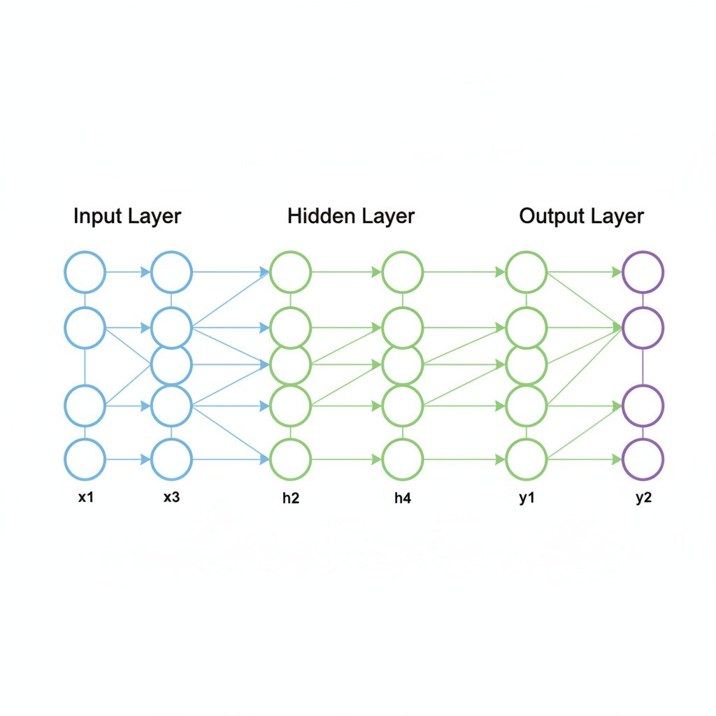
The simplest form of a deep neural network is called a Multi-Layer Perceptron (MLP). It’s typically composed of three types of layers:

1. The Input Layer: This isn’t a true layer of computation. It simply represents our initial data vector. If we’re analyzing a 784-pixel image, the input layer has 784 nodes, each holding the value of one pixel.
2. The Hidden Layer(s): This is where the magic happens. A hidden layer is a collection of neurons that sits between the input and output layers. Each neuron in a hidden layer is connected to all the nodes in the previous layer. A “deep” neural network is simply one that has multiple hidden layers.
3. The Output Layer: This is the final layer of neurons that produces the network’s prediction. The number of neurons in this layer depends on the task:
   • For regression (predicting a price), it might be a single neuron.
   • For binary classification (Cat vs. Dog), it might be a single neuron with a Sigmoid activation.
   • For multi-class classification (Cat vs. Dog vs. Bird), it would have multiple neurons, one for each class.

The Flow of Information: A Cascade of Transformations

Let’s trace how a piece of data flows through a simple network with one hidden layer.

1. Input to Hidden Layer:
   • The input vector is fed into the network.
   • To calculate the pre-activation value for the first neuron in the hidden layer, we perform a dot product between the entire input vector and the specific weight vector that connects the input layer to that one neuron. A bias is added.
   • We repeat this for every neuron in the hidden layer. Each neuron has its own unique set of weights.
   • This entire operation, for the whole layer, can be represented efficiently as a single matrix multiplication: (Input Vector * Weight Matrix) + Bias Vector.
   • The result is a new vector of weighted sums, one for each neuron in the hidden layer.
2. Activation:
   • This vector of weighted sums is then passed through a non-linear activation function, like ReLU. Each element of the vector is processed by the ReLU function (max(0, x)).
   • The output is a new vector, the “activation vector” of the hidden layer.
3. Hidden Layer to Output Layer:
   • This activation vector from the hidden layer now becomes the input for the next layer (the output layer).
   • The process repeats: we perform another matrix multiplication using the output layer’s weight matrix, add a bias, and apply a final activation function (e.g., Sigmoid for classification) to get the network’s final prediction.

Learning Progressively More Complex Features

Why is this layered structure so powerful? Because it allows the network to learn a hierarchy of features.

Imagine an image recognition task:

• The first hidden layer, which looks directly at the raw pixels, might learn to recognize very simple features: edges, corners, simple color gradients. Its neurons will activate when they “see” these basic components.
• The second hidden layer doesn’t see the pixels. It sees the output of the first layer. It takes the simple features (edges, corners) as input and learns to combine them into more complex shapes: eyes, ears, noses, whiskers.
• A third hidden layer might take these shapes as input and learn to combine them into even more complex concepts: “cat face,” “dog snout.”
• Finally, the output layer takes these high-level feature representations and makes the final decision: “The combination of features I’m seeing is most consistent with the label ‘Cat’.”

Each layer is a transformation that takes the representation from the previous layer and converts it into a slightly more abstract and useful representation. The network automatically learns the best features to look for at each level of abstraction, all guided by the single goal of minimizing the final cost function via Gradient Descent and Backpropagation.

This is the power of stacking simple neurons into deep layers. It’s a modular, hierarchical system that can take raw, low-level data and, through a series of learned transformations, build up a rich, high-level understanding of the world.