Lecture 38: The Perceptron: The “Single Neuron” that Started It All

Series: The Sequentia Lectures: Unlocking the Math of AI
Part 5: Core Machine Learning in Action
Lecture 38: The Perceptron: The “Single Neuron” that Started It All

We’ve built models that can draw lines (Linear Regression) and predict probabilities (Logistic Regression). Now, we’re going to take a step back in history and forward in concept to meet the ancestor of all modern neural networks: the Perceptron.

Developed in the 1950s by Frank Rosenblatt, the Perceptron was a groundbreaking attempt to create a computational model of a biological neuron. While simple by today’s standards, its core design provides the fundamental intuition for how every single neuron in a deep neural network operates. It’s the “atom” of the AI brain.

The Anatomy of a Single Artificial Neuron

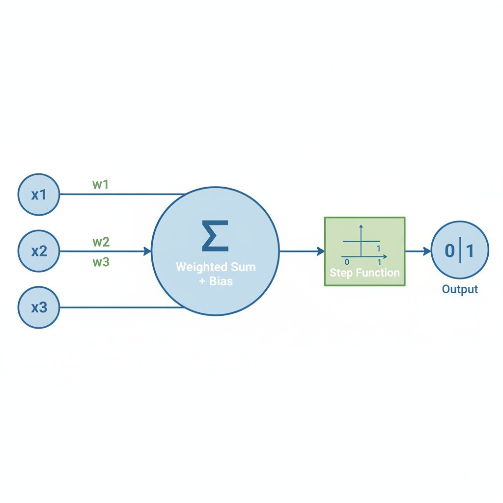
A Perceptron is a simple decision-making unit. It takes several numerical inputs and produces a single binary output (0 or 1, Yes or No). Here’s how it works, step by step:

1. Inputs (x₁, x₂, x₃, …): The neuron receives one or more numerical inputs. These could be the raw pixel values of an image, features of a dataset, or the outputs from other neurons.
2. Weights (w₁, w₂, w₃, …): Each input is assigned a weight. The weight represents the “importance” of that specific input.
   • A large positive weight means this input is a strong signal in favor of the neuron “firing.”
   • A large negative weight means this input is a strong signal against the neuron “firing.”
   • A weight close to zero means the input is largely irrelevant.
3. The Weighted Sum (Dot Product!): The Perceptron calculates a weighted sum of all its inputs. It multiplies each input by its corresponding weight and adds them all up. Does this sound familiar? It’s exactly the dot product of the input vector and the weight vector!
   Sum = (x₁ * w₁) + (x₂ * w₂) + (x₃ * w₃) + …
   Often, a bias term (b) is also added to this sum. The bias acts as an “offset,” making it easier or harder for the neuron to fire, independent of its inputs.
   Sum = (x₁ * w₁) + (x₂ * w₂) + … + b
4. The Activation Function (A Simple Step): The Perceptron takes this final sum and passes it through an activation function to make a decision. The original Perceptron used a simple step function.
   • If Sum > 0 (or some other threshold), the neuron “fires” and outputs 1.
   • If Sum <= 0, the neuron does not fire and outputs 0.

An Intuitive Example: To Go to the Beach or Not?

Let’s model a simple decision. Should you go to the beach? Your decision (fire = 1, don’t fire = 0) depends on three inputs:

• x₁: Is the weather sunny? (1 for Yes, 0 for No)
• x₂: Do you have friends going? (1 for Yes, 0 for No)
• x₃: Is it a weekday? (1 for Yes, 0 for No)

You assign weights based on your preferences:

• w₁ = 6 (Sunny weather is very important)
• w₂ = 3 (Friends going is a nice bonus)
• w₃ = -5 (Weekdays are a strong negative factor, as you have to work)
• Let’s set a bias b = -2. This represents your general slight reluctance to go unless conditions are good.

Now, let’s say it’s a sunny weekday, and your friends are going: Inputs = [1, 1, 1]
Sum = (1 * 6) + (1 * 3) + (1 * -5) + (-2) = 6 + 3 – 5 – 2 = 2
Since Sum (2) > 0, the Perceptron fires. Output = 1 (Go to the beach!).

What if it’s a sunny weekend and your friends are going? Inputs = [1, 1, 0] (weekday is 0)
Sum = (1 * 6) + (1 * 3) + (0 * -5) + (-2) = 6 + 3 – 0 – 2 = 7
Since Sum (7) > 0, the Perceptron fires. Output = 1 (Definitely go!).

Learning: The Perceptron Learning Rule

How does a Perceptron learn the right weights? The original learning rule was simple and iterative:

1. Start with random weights.
2. Feed it a training example.
3. If the prediction is correct, do nothing.
4. If the prediction is wrong:
   • If it predicted 0 but should have been 1, slightly increase the weights associated with the active inputs.
   • If it predicted 1 but should have been 0, slightly decrease the weights associated with the active inputs.
5. Repeat for all training examples, over and over.

This simple rule allows the Perceptron to gradually nudge its weights until it finds a combination that correctly separates the data.

The Bridge to Modern Neural Networks

The Perceptron is the direct ancestor of the neurons used in today’s deep networks. The core idea—a weighted sum followed by an activation function—is identical. The main difference is that modern neurons replace the harsh step function with smoother, differentiable functions (like the Sigmoid from our last lecture!), which allows us to use the power of Gradient Descent and the Chain Rule (Backpropagation) to train them much more effectively.

By understanding this single, simple computational unit, you’ve understood the fundamental building block of even the most complex neural networks in the world.