Lecture 41: Backpropagation Explained: How Errors Flow Backwards to Teach the Network

Series: The Sequentia Lectures: Unlocking the Math of AI
Part 5: Core Machine Learning in Action
Lecture 41: Backpropagation Explained: How Errors Flow Backwards to Teach the Network

We’ve built a neural network. It takes an input, passes it forward through a series of layers, and makes a final prediction. But if that prediction is wrong—and at the start of training, it will be wildly wrong—how does the network learn from its mistake? How do the weights in the very first layer know how they contributed to the final error?

The answer is a beautiful and efficient algorithm called Backpropagation. It’s the engine of learning in deep learning, and while the name sounds complex, the core idea is an elegant application of concepts we’ve already learned: the Cost Function, Gradients, and especially the Chain Rule.

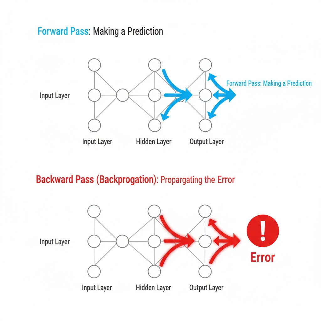
The Forward Pass: Making a Guess

First, let’s remember the “forward pass.” Our input data (e.g., an image vector) flows forward through the network:
Input -> Layer 1 -> Layer 2 -> … -> Final Output (Prediction)
Each step is a matrix multiplication followed by an activation function.

Step 1: Calculating the Final Error

At the very end, we compare the network’s Prediction to the True Answer using our Cost Function (like Cross-Entropy or MSE). This gives us a single number: the total Error.

This is our starting point. We know the total error, but we don’t know who to “blame.” How much did each of the millions of weights in the network contribute to this final error?

Step 2: The Backward Pass – Assigning Blame with the Chain Rule

This is where Backpropagation begins. It works backwards from the final error, layer by layer, distributing the “blame” and calculating the gradient for every weight.

1. At the Output Layer:
   • Backpropagation first calculates the partial derivative of the Error with respect to the output of the final layer. This is a direct, one-step calculation. It tells us: “How did the final neuron’s activation affect the total error?”
2. Moving to the Last Hidden Layer:
   • Now comes the Chain Rule (from Lecture 17). We want to know how the weights in the last hidden layer affected the error. We do this by “chaining” the derivatives:
     • We know how the final layer’s output affected the error.
     • We can calculate how the last hidden layer’s weights affected the final layer’s output.
   • By multiplying these two rates of change, the Chain Rule gives us the derivative we need: the influence of the last hidden layer’s weights on the final error.
3. Propagating to Deeper Layers:
   • The process repeats. The error signal is “propagated” further backward. To find the gradient for the weights in the second-to-last hidden layer, we chain together the influence of that layer on the last hidden layer, and the influence of the last hidden layer on the error.
   • This continues, step by step, all the way back to the very first hidden layer.

An Intuition: The Multi-Stage Rocket

Imagine a multi-stage rocket trying to hit a target. The final position error is caused by tiny misalignments in every stage that fired before it.

• The final stage’s error is easy to calculate.
• To figure out the first stage’s contribution, you need to know how the first stage’s firing affected the second stage’s trajectory, how the second affected the third, and how the third affected the final position.
• Backpropagation is like using the Chain Rule to trace this cascade of influence in reverse, from the final error back to the initial launch parameters.

Step 3: Updating the Weights with Gradient Descent

Once Backpropagation has completed its journey from the last layer to the first, it has computed the partial derivative of the error with respect to every single weight in the entire network.

We now have our complete gradient vector.

From here, it’s just Gradient Descent as we know it! We use this gradient to update all the weights, taking a small step in the opposite direction to reduce the overall error.

new_weight = old_weight – (learning_rate * gradient_for_that_weight)

The Complete Learning Cycle

The entire training process for a neural network is a continuous loop of these two passes:

1. Forward Pass: Feed the data through, make a prediction.
2. Calculate Error: Compare the prediction to the truth.
3. Backward Pass (Backpropagation): Calculate the gradient of the error with respect to every weight by propagating the error signal backwards using the Chain Rule.
4. Update Weights: Use Gradient Descent to adjust all weights slightly.
5. Repeat with the next batch of data.

Backpropagation is the computational shortcut that makes this possible. It’s a clever, recursive application of the Chain Rule that allows us to efficiently calculate the gradient for millions of parameters, turning the “magic” of deep learning into a concrete, step-by-step optimization problem.