Series: The Sequentia Lectures: Unlocking the Math of AI
Part 3: The AI Toolkit: Calculus & Optimization
Lecture 22: Learning Rate: The Art of Taking Steps of the Right Size
In our last lecture, we unveiled the engine of AI learning: Gradient Descent. The strategy is simple: find the steepest way downhill in our error landscape and take a step. We repeat this until we find the bottom of the valley.
But this leaves one crucial, unanswered question: How big should our steps be?
This “step size” is a critical setting in training an AI, a “hyperparameter” that we must choose. It’s called the learning rate. Getting it right is an art, and it involves a delicate trade-off. Too big or too small, and our journey to the optimal solution can fail.
The Learning Rate: Our Stride Length
Think back to our analogy of being lost in a foggy valley. The learning rate is your stride length. You’ve used the gradient to figure out the downhill direction, but you still have to decide how far to move with each step.
new_weight = old_weight – (learning_rate * gradient_component)
The learning_rate is a small positive number (e.g., 0.1, 0.01, or 0.001) that multiplies the gradient. It scales the size of our update. Let’s explore what happens when we choose our stride length poorly.
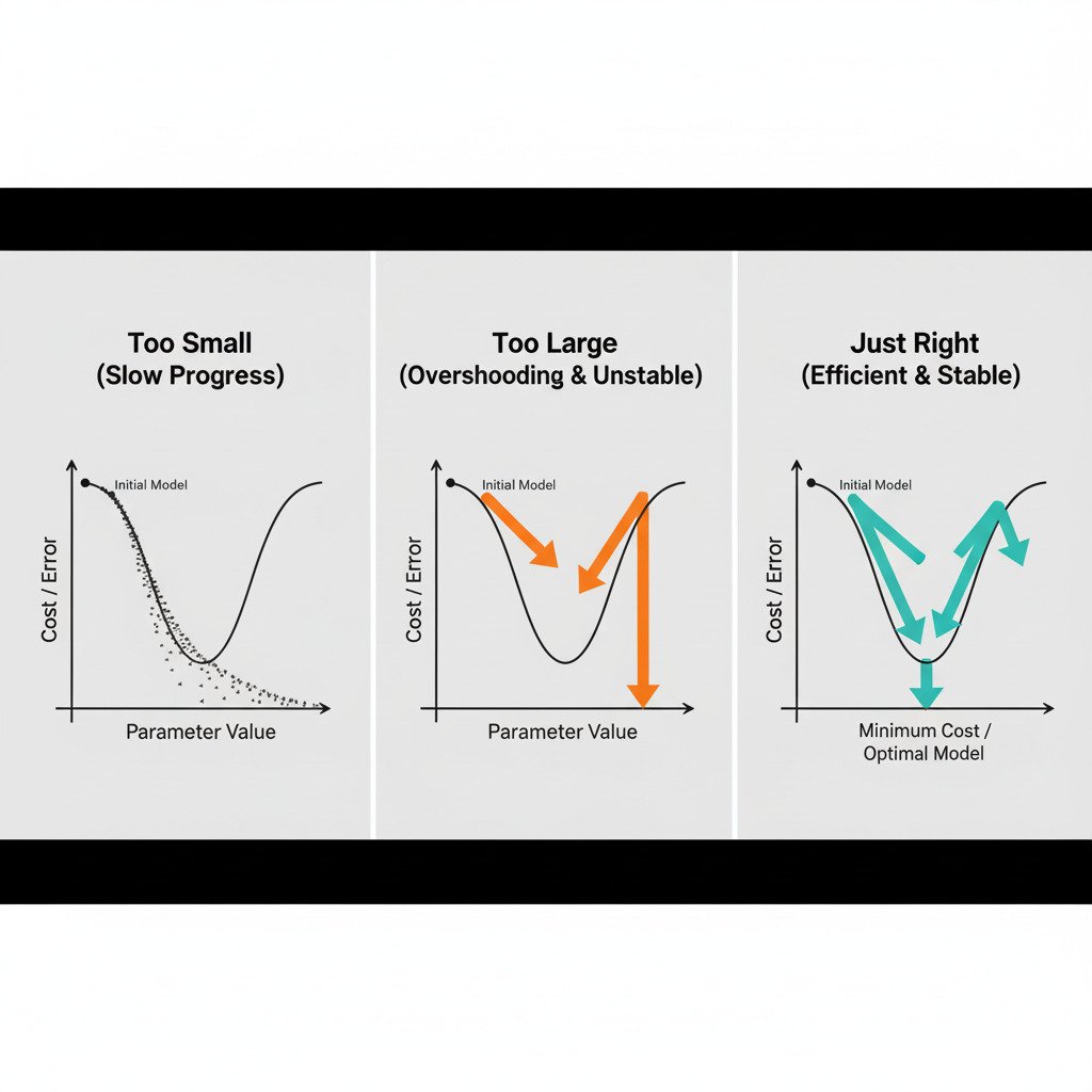
Scenario 1: The Learning Rate is Too Small (Timid Steps)
Imagine setting your stride length to just a few centimeters. You meticulously find the downhill direction and then take a tiny shuffle forward. You repeat this, shuffling again and again.
- The Good: You are almost guaranteed to never miss the bottom of the valley. Your path will be very smooth and precise.
- The Bad: It will take an incredibly long time to get there! If the valley is large, you might spend ages taking millions of tiny, inefficient steps.
- In AI Terms: A learning rate that’s too small leads to extremely slow training. The model will improve, but the convergence to the optimal set of parameters will be painfully slow, costing valuable time and computational resources.
Scenario 2: The Learning Rate is Too Large (Reckless Leaps)
Now, imagine setting your stride length to a giant leap. You find the downhill direction and take a huge bound.
- The Problem: You might completely overshoot the bottom of the valley and land on the other side, possibly even higher up than where you started! From your new, higher position, you calculate the new downhill direction (which is now back the way you came) and take another giant leap, overshooting the minimum again.
- The Result: You bounce erratically from one side of the valley to the other, either making very slow progress or, in the worst case, getting further and further away from the solution. The error might jump around wildly and never decrease.
- In AI Terms: A learning rate that’s too large can cause the training process to become unstable and diverge. The cost function won’t decrease; it might oscillate or even increase. The model fails to learn.
Scenario 3: The “Goldilocks” Learning Rate (Just Right)
The ideal learning rate is like a confident but careful stride. It’s large enough to make meaningful progress down the slope in a reasonable amount of time, but small enough that it doesn’t overshoot the minimum.
- The Path: You take large steps when the slope is steep (when the gradient is large) and naturally smaller steps as the ground flattens out near the bottom of the valley (as the gradient approaches zero). You efficiently descend and settle smoothly into the minimum.
- In AI Terms: A well-chosen learning rate leads to efficient and stable training. The cost function decreases steadily, and the model converges to a good solution in a timely manner.
The Art of Hyperparameter Tuning
Finding this “Goldilocks” learning rate is a central task in applied machine learning, known as hyperparameter tuning. There is no single magic number that works for all problems. Data scientists and AI engineers often experiment with different values, use automated techniques, or employ more advanced “adaptive learning rate” algorithms (like Adam or RMSprop) that can automatically adjust the step size during training.
This concludes our foundational tour of Calculus & Optimization for AI! We’ve learned how to quantify our model’s error with a Cost Function and how to systematically minimize that error using the elegant algorithm of Gradient Descent, guided by the all-important learning rate.
With a solid understanding of both Linear Algebra and Calculus, we are now truly ready to build and understand our first predictive model.
