Series: The Sequentia Lectures: Unlocking the Math of AI
Part 3: The AI Toolkit: Calculus & Optimization
Lecture 20: Introducing the Cost Function: Quantifying “How Wrong” Our Model Is
We’ve spent the last few lectures assembling a powerful toolkit. We know our AI model is a function, f(x) = y, that makes predictions. We know we want to improve it. We even have a compass—the gradient—that tells us which way to adjust our model’s parameters to get better.
But what, exactly, are we trying to improve? How do we measure “better” or “worse”? Before we can begin our journey “downhill” into the valley of a perfect solution, we first need a way to map out the landscape. We need a way to quantify, with a single, precise number, exactly how wrong our model currently is.
This is the job of the Cost Function (also known as a Loss Function or Error Function).
The Cost Function: A Measure of Pain
A cost function is a mathematical formula that compares our model’s predictions to the actual, ground-truth answers and calculates a single numerical score representing the total error or “cost.”
Think of it as a measure of “pain.” The higher the cost, the more “pain” the model is in because its predictions are far from the truth. The lower the cost, the better the model is performing.
The entire goal of the training process is to find the set of model parameters (weights) that minimizes the value of this cost function.
How Does It Work?
Let’s imagine a simple model that tries to predict a house’s price. For a single house, we have:
- The True Price (the ground truth, y): $300,000
- Our Model’s Prediction (the predicted output, ŷ, often called “y-hat”): $250,000
Our model is off by $50,000. This difference is the error for a single data point. The cost function’s job is to aggregate these individual errors from all the data points in our training set into one overall score.
An Example: Mean Squared Error (MSE)
One of the most common cost functions for prediction problems (like predicting prices) is the Mean Squared Error (MSE). It sounds complicated, but the process is straightforward:
- Calculate the Error: For each data point, find the difference between the prediction and the true value (prediction – true_value).
- Square the Error: Square this difference. This does two important things: it makes all errors positive (so that being too high or too low both contribute to the cost), and it penalizes larger errors much more heavily than smaller ones. A $50,000 error is much worse than five $10,000 errors.
- Calculate the Mean (Average): Add up all the squared errors from every data point in your dataset and then divide by the total number of data points.
This final number, the MSE, is our total cost. It’s a single, scalar value that tells us, on average, how badly our model is performing across the entire dataset.
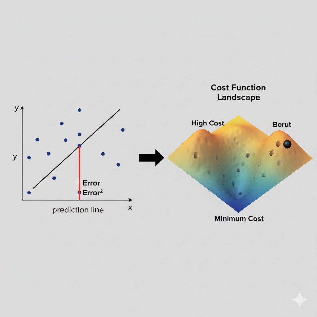
The Shape of the Landscape
The cost function is what defines the error landscape we’ve been discussing.
- The inputs to the cost function are the model’s parameters (weights).
- The output is the cost (the error).
If we imagine a simple model with just two weights, we can visualize the cost function as a 3D surface. Some combinations of the two weights will result in a high cost (a high peak on the landscape), while other combinations will result in a low cost (a deep valley).
The job of our optimization algorithm (Gradient Descent, which we’ll cover next) is to navigate this landscape, using the gradient of the cost function as its guide, to find the coordinates (the specific values of the weights) that correspond to the lowest point in this valley.
The cost function, therefore, is the ultimate arbiter of success. It’s the judge that scores our model’s performance, providing the concrete, quantifiable feedback our AI needs to begin the iterative process of learning from its mistakes. Without a way to measure “wrong,” there can be no path to “right.”
