Series: The Sequentia Lectures: Unlocking the Math of AI
Part 4: The AI Toolkit: Probability & Statistics
Lecture 32: Maximum Likelihood Estimation: Finding the Best Explanation for What We See
Imagine you are a detective who has just arrived at the scene of a crime. You have a set of clues—the “data.” Your job is to find the suspect whose story makes the observed clues “most likely” to have occurred. You’d consider different suspects (your “models”) and evaluate how well their proposed scenarios explain the evidence.
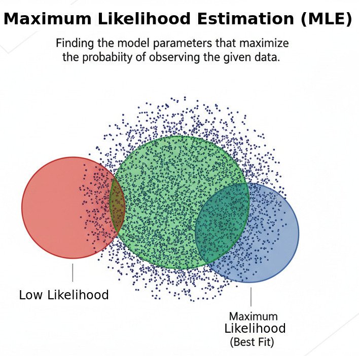
This process of working backwards from observed data to find the most plausible underlying model is a powerful statistical principle known as Maximum Likelihood Estimation (MLE). It’s a fundamental method for “fitting” a model to data and is the conceptual foundation for many of the cost functions we use in machine learning.
The Core Idea: Which Model Makes My Data Least Surprising?
Let’s use a simpler example. Imagine you flip a coin 10 times and get the following sequence:
Heads, Heads, Tails, Heads, Heads, Heads, Tails, Heads, Heads, Heads (8 Heads, 2 Tails)
You don’t know if the coin is fair. You want to find the best possible model for this coin. A “model” for a coin is simply its probability of landing on heads, a parameter we’ll call p.
- Model A (Fair Coin): p = 0.5
- Model B (Biased Coin): p = 0.8
- Model C (Very Biased Coin): p = 0.2
Which model is the “best” explanation for the data we just saw? Maximum Likelihood Estimation asks: Under which model is the probability (the “likelihood”) of observing our specific data sequence the highest?
Let’s calculate the likelihood for each model:
- Likelihood under Model A (p=0.5): The probability of getting this specific sequence (8 heads, 2 tails) with a fair coin is 0.5⁸ * 0.5² ≈ 0.00097. This is a very unlikely, or “surprising,” outcome for a fair coin.
- Likelihood under Model B (p=0.8): The probability of getting this sequence with a coin biased towards heads is 0.8⁸ * 0.2² ≈ 0.0067. This outcome is more likely under this model.
- Likelihood under Model C (p=0.2): The probability is 0.2⁸ * 0.8² ≈ 0.0000016. This outcome is extremely surprising for a coin biased towards tails.
Comparing the likelihoods, Model B (p=0.8) makes our observed data most likely or least surprising. Therefore, according to the principle of Maximum Likelihood Estimation, p=0.8 is the best estimate for our coin’s true probability of heads. We have “fit” the model to the data.
From Coin Flips to AI Models
This same principle applies to complex AI models. Let’s consider a simple linear model trying to find the best-fit line through a scatter plot of data.
- Data: A set of (x, y) points.
- Model: A line, defined by its parameters (slope m and intercept b).
- MLE Question: Which possible line (which combination of m and b) makes the observed (x, y) data points most likely to have occurred?
We assume that our data points follow the line’s prediction but with some random “noise,” which we often assume follows a Normal (Gaussian) distribution. The MLE process then becomes a search. It “tries on” millions of different lines. For each line, it calculates the likelihood of our data points appearing where they did. The line that results in the maximum possible likelihood is chosen as the best fit.
The Connection to Cost Functions
Here’s the beautiful connection: it turns out that for many common assumptions (like normally distributed noise), maximizing the likelihood is mathematically equivalent to minimizing a cost function like the Mean Squared Error (MSE) that we discussed in Lecture 20!
When we use Gradient Descent to find the parameters that minimize the MSE, we are, in fact, also finding the parameters that maximize the likelihood of our data. The principle of MLE provides the deep, statistical justification for why minimizing that specific cost function is the right thing to do.
Maximum Likelihood Estimation gives us a powerful, universal framework for model fitting. It turns the art of “choosing a model” into a formal optimization problem: find the parameters that provide the best possible explanation for the data we see. It’s the statistical engine that drives our AI’s search for the “truth” hidden in the data.
