Series: The Sequentia Lectures: Unlocking the Math of AI
Part 4: The AI Toolkit: Probability & Statistics
Lecture 29: Probability Distributions: Describing the Shape of Uncertainty (Gaussian/Normal)
So far, we’ve discussed probability as the likelihood of a single event, like rolling a 4 on a die. But in data science, we’re rarely interested in just one outcome. We want to understand the entire landscape of possibilities. What is the probability of all possible outcomes?
The mathematical tool for describing this is a probability distribution. It’s a function or a graph that tells us the probability of every possible result of a random event. It gives us the “shape” of our uncertainty.
Discrete vs. Continuous Distributions
There are many types of distributions, but they generally fall into two categories:
- Discrete Distributions: Used when the outcomes are distinct, countable values. The roll of a die is a discrete event; the outcomes are {1, 2, 3, 4, 5, 6}. You can’t roll a 2.5. We can represent this with a bar chart, where each bar’s height is the probability of that specific outcome (1/6 for each bar in a fair die roll).
- Continuous Distributions: Used when the outcome can be any value within a given range. Human height is a continuous variable; you can be 175cm, 175.1cm, or 175.11cm tall. We represent these with a smooth curve, where the area under the curve between two points represents the probability of the outcome falling within that range.
The Star of the Show: The Normal (Gaussian) Distribution
Among all the continuous distributions, one reigns supreme in its importance and prevalence: the Normal Distribution, also known as the Gaussian Distribution or, more colloquially, the Bell Curve.
You’ve undoubtedly seen its iconic, symmetric, bell-like shape. It’s defined by two key parameters:
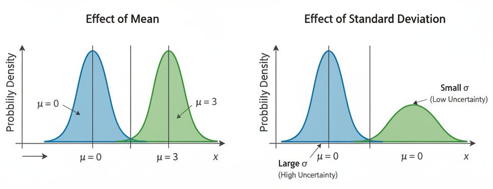
- The Mean (μ): This is the center of the bell, representing the average or most likely value. The peak of the curve is always at the mean.
- The Standard Deviation (σ): This measures the “spread” or “width” of the bell.
- A small standard deviation results in a tall, narrow curve, meaning most data points are clustered very tightly around the mean. There is low uncertainty.
- A large standard deviation results in a short, wide curve, meaning the data points are spread out over a larger range. There is high uncertainty.
Why is the Bell Curve Everywhere? The Central Limit Theorem
The Normal distribution isn’t just a neat mathematical construct; it’s a fundamental pattern of the universe. Why? The main reason is a remarkable mathematical law called the Central Limit Theorem (CLT).
In simple terms, the CLT states that if you take a large number of independent random variables and add them together, the distribution of their sum (or average) will tend to look like a Normal distribution, regardless of the original distribution of the individual variables.
Think about it: a person’s height is the result of thousands of tiny, independent genetic and environmental factors all added together. The final measurement on a test is the sum of many small factors (how well you slept, what you ate, which questions you knew, etc.). Stock market fluctuations are the sum of millions of individual buying and selling decisions.
Because so many phenomena in the real world are the aggregate result of many small, random influences, their distributions naturally converge to the bell curve. This makes it an incredibly powerful tool for modeling the world.
The Normal Distribution in AI
In machine learning, we use the Normal distribution constantly:
- Initializing Models: When we first create a neural network, we don’t know what the initial weights should be. A common practice is to initialize them by drawing random numbers from a Normal distribution centered at zero.
- Modeling Noise: We often assume that the “noise” or random error in our data follows a Normal distribution. This assumption allows us to make statistically sound judgments about our model’s performance.
- Generating Data: In some types of generative AI, we can sample from a learned Normal distribution to create new, realistic-looking data points that resemble our training data.
- Statistical Inference: It’s the foundation for many statistical tests that help us determine if our model’s findings are significant or just the result of random chance.
A probability distribution, and the Normal distribution in particular, gives us a powerful lens through which to view our data. It allows us to move beyond individual data points and begin to understand the underlying structure, patterns, and inherent uncertainty of the entire dataset. It provides the “shape” of the landscape that our AI models will learn to navigate.
