Series: The Sequentia Lectures: Unlocking the Math of AI
Part 4: The AI Toolkit: Probability & Statistics
Lecture 28: Bayes’ Theorem: The Mathematical Heart of “Learning from Evidence”
In our last lecture, we saw how conditional probability allows us to update our beliefs when we get new information. P(A | B) tells us the probability of A, given B is true.
But what if we know P(B | A) and want to find P(A | B)? This “flipping” of the condition is an incredibly common and powerful form of reasoning, and it’s governed by one of the most celebrated and important formulas in all of probability theory: Bayes’ Theorem.
Bayes’ Theorem is the mathematical engine of “learning from evidence.” It provides a formal recipe for updating a hypothesis based on observed data.
The Famous Formula
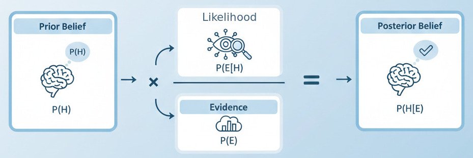
Let’s look at the theorem first, and then break it down with an intuitive example. For a hypothesis H and some observed evidence E, Bayes’ Theorem is:
P(H | E) = [ P(E | H) * P(H) ] / P(E)
It looks intimidating, but each piece has a simple, common-sense name and role:
- P(H | E) – Posterior Probability: What we want to find. The probability of our hypothesis H being true, after we have seen the evidence E. This is our updated belief.
- P(E | H) – Likelihood: The probability of seeing the evidence E, assuming that our hypothesis H is true. How likely is this evidence, given our theory?
- P(H) – Prior Probability: The probability of our hypothesis H being true, before we saw any evidence. This is our initial belief or “prior.”
- P(E) – Marginal Likelihood: The overall probability of seeing the evidence E, regardless of whether the hypothesis is true or not. This acts as a normalization constant.
So, the theorem can be stated in words as:
Posterior Belief = (Likelihood of Evidence given Belief * Prior Belief) / Overall Likelihood of Evidence
An Intuitive Example: The Medical Test
Let’s say there’s a rare disease that affects 1% of the population. There’s a test for this disease that is 99% accurate (if you have the disease, it will be positive 99% of the time; if you don’t, it will be negative 99% of the time).
You take the test, and it comes back positive. What is the actual probability that you have the disease?
Our intuition might scream “99%!”, but let’s use Bayes’ Theorem to find the real answer.
- Hypothesis (H): You have the disease.
- Evidence (E): Your test is positive.
- We want to find: P(H | E) – The probability you have the disease, given that you tested positive.
Let’s find the pieces:
- P(H) (Prior): The probability of having the disease before any evidence. We know this is 1% of the population, so P(H) = 0.01.
- P(E | H) (Likelihood): The probability of testing positive, assuming you have the disease. This is the test’s accuracy, so P(E | H) = 0.99.
- P(E) (Overall Evidence): This is the trickiest part. What’s the overall probability of anyone testing positive? This can happen in two ways:
- A person has the disease AND tests positive (a true positive).
- A person does NOT have the disease AND tests positive (a false positive).
- P(E) = P(true positive) + P(false positive)
- P(true positive) = P(H) * P(E | H) = 0.01 * 0.99 = 0.0099
- P(false positive) = P(not H) * P(E | not H) = 0.99 * 0.01 = 0.0099 (99% of people don’t have the disease, and the test is wrong 1% of the time for them).
- P(E) = 0.0099 + 0.0099 = 0.0198.
Now, let’s plug it all into Bayes’ Theorem:
P(H | E) = [ P(E | H) * P(H) ] / P(E)
P(H | E) = [ 0.99 * 0.01 ] / 0.0198
P(H | E) = 0.0099 / 0.0198 = 0.5
The result is 50%. Despite a 99% accurate test, your probability of actually having the disease is only 50%! Why? Because the disease is so rare (your “prior” was so low) that a false positive is just as likely as a true positive. Your strong prior belief (“I probably don’t have this rare disease”) was correctly updated by the evidence, but not completely overturned.
Bayes’ Theorem as the Core of Learning
This process is the essence of “Bayesian inference,” a major field within machine learning.
- An AI model starts with a “prior” belief about its parameters.
- As it sees each new piece of data (“evidence”), it uses Bayes’ Theorem to update its beliefs, turning its “prior” into a “posterior.”
- This new posterior then becomes the “prior” for the next piece of data it sees.
This iterative updating is a formal, powerful way of learning from experience. It’s used in spam filters (updating the probability of “spam” given the evidence of certain words), medical diagnostics, and many other AI systems that need to reason and make decisions under uncertainty. Bayes’ Theorem provides the elegant, mathematical recipe for how to blend our old knowledge with new evidence to arrive at a more refined truth.
