Series: The Sequentia Lectures: Unlocking the Math of AI
Part 3: The AI Toolkit: Calculus & Optimization
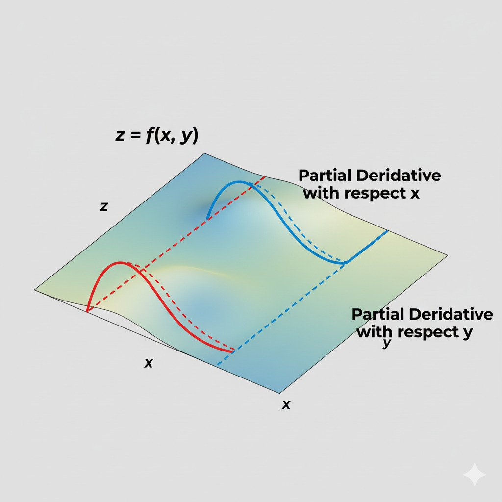
Lecture 18: Functions with Many Inputs: Thinking in Partial Derivatives
So far, when we’ve talked about derivatives, we’ve used a simple analogy: standing on a 2D hillside where our position is a single number x and the height is the output f(x). The derivative tells us the slope in that one possible direction of movement (along the x-axis).
But our AI models are far more complex. The “error function” of a neural network doesn’t have just one input; it has millions of inputs—one for every single weight and parameter in the model. Its landscape isn’t a 2D hill; it’s a mind-bogglingly complex surface in millions of dimensions.
How can we possibly find the “slope” in such a space? We do it by simplifying the problem, using a tool called the partial derivative.
The Partial Derivative: Isolating One Variable at a Time
The core idea behind a partial derivative is simple and elegant: if you have a function with many inputs, just pretend that all but one of them are temporarily frozen in place.
Imagine you’re standing on a real mountain. Your elevation depends on two inputs: your longitude (East/West position) and your latitude (North/South position). You want to know the slope. But the “slope” isn’t a single number!
- The slope in the pure North direction might be steeply uphill.
- The slope in the pure East direction might be gently downhill.
A partial derivative is what you calculate when you ask about the slope in only one of these specific directions.
- The partial derivative with respect to latitude tells you the slope if you only move North/South, holding your East/West position constant.
- The partial derivative with respect to longitude tells you the slope if you only move East/West, holding your North/South position constant.
You’ve turned a complex 3D slope problem into two simpler 2D slope problems.
From Mountains to Models
Now, let’s apply this to our AI model’s error function. This function’s inputs are all the model’s parameters: Weight₁, Weight₂, Weight₃, …, Weight₁₀₀₀₀₀₀. The output is the total error.
We want to know how to adjust these weights to reduce the error. To do this, we calculate the partial derivative of the error with respect to each weight individually.
- Calculate for Weight₁: We find the partial derivative of the error with respect to Weight₁. This tells us: “If we hold all other 999,999 weights perfectly still and just nudge Weight₁ a tiny bit, how will the total error change?” This gives us the “slope” in the Weight₁ direction.
- Calculate for Weight₂: We repeat the process, finding the partial derivative of the error with respect to Weight₂. This tells us the slope in the Weight₂ direction.
- …and so on for all one million weights.
This is exactly what the Backpropagation algorithm (which we learned uses the Chain Rule) does. It efficiently calculates the partial derivative of the final error with respect to every single parameter in the entire network.
The Gradient: A Vector of All Slopes
After we’ve calculated all these individual partial derivatives, we can assemble them into a single, powerful object: a gradient.
A gradient is simply a vector where each element is the partial derivative with respect to one of the input parameters.
Gradient of Error = [ (partial derivative wrt W₁), (partial derivative wrt W₂), … ]
This gradient vector is amazing. It’s a single arrow in our multi-million-dimensional error landscape that points in the direction of the steepest possible ascent. It combines all the individual “slopes” to tell us the single best direction to move in order to increase the error as quickly as possible.
And if we want to decrease the error (which is always our goal), we just take a small step in the exact opposite direction of the gradient. This process is called Gradient Descent, and it is the fundamental optimization algorithm for training almost all modern AI models. We’ll explore it in detail in our next lecture.
The partial derivative, therefore, is the tool that allows us to manage overwhelming complexity. It lets us break down a problem with millions of moving parts into a million simple questions, and the gradient assembles the answers into one clear, actionable instruction: “This way to the bottom of the valley.”
